

Prepara tus exámenes y mejora tus resultados gracias a la gran cantidad de recursos disponibles en Docsity

Gana puntos ayudando a otros estudiantes o consíguelos activando un Plan Premium


Prepara tus exámenes
Prepara tus exámenes y mejora tus resultados gracias a la gran cantidad de recursos disponibles en Docsity
Prepara tus exámenes con los documentos que comparten otros estudiantes como tú en Docsity
Los mejores documentos en venta realizados por estudiantes que han terminado sus estudios
Estudia con lecciones y exámenes resueltos basados en los programas académicos de las mejores universidades
Responde a preguntas de exámenes reales y pon a prueba tu preparación

Consigue puntos base para descargar
Gana puntos ayudando a otros estudiantes o consíguelos activando un Plan Premium
Comunidad
Pide ayuda a la comunidad y resuelve tus dudas de estudio
Descubre las mejores universidades de tu país según los usuarios de Docsity
Ebooks gratuitos
Descarga nuestras guías gratuitas sobre técnicas de estudio, métodos para controlar la ansiedad y consejos para la tesis preparadas por los tutores de Docsity
Examples and information about functions of several variables
Tipo: Resúmenes
1 / 9

Esta página no es visible en la vista previa
¡No te pierdas las partes importantes!


In this section we want to go over some of the basic ideas about functions of more than one variable.
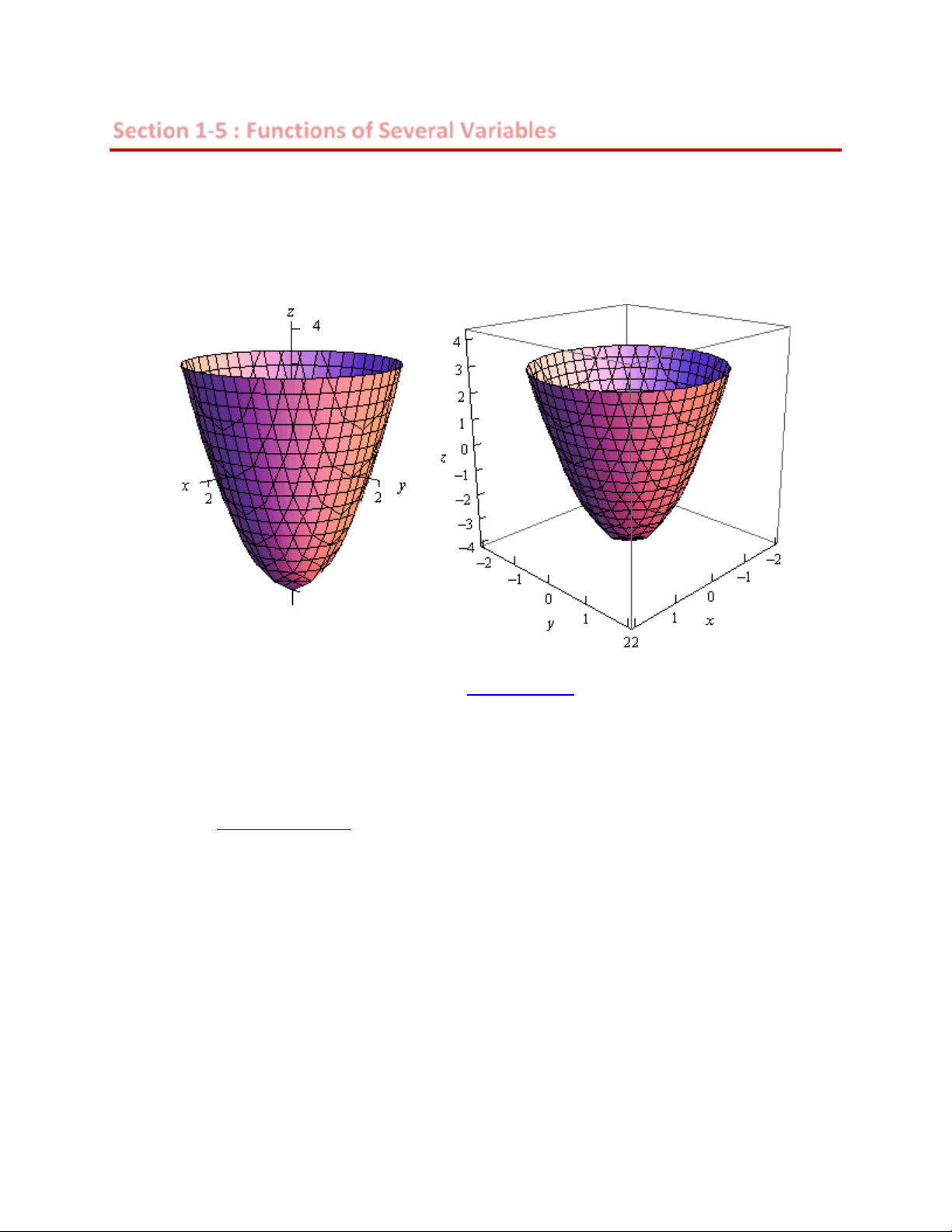
dimensional space. For example, here is the graph of z = 2 x^2^ + 2 y^2 − 4.
This is an elliptic paraboloid and is an example of a quadric surface. We saw several of these in the previous section. We will be seeing quadric surfaces fairly regularly later on in Calculus III.
Another common graph that we’ll be seeing quite a bit in this course is the graph of a plane. We have a convention for graphing planes that will make them a little easier to graph and hopefully visualize.
Recall that the equation of a plane is given by
ax + by + cz = d
or if we solve this for z we can write it in terms of function notation. This gives,
To graph a plane we will generally find the intersection points with the three axes and then graph the triangle that connects those three points. This triangle will be a portion of the plane and it will give us a fairly decent idea on what the plane itself should look like. For example, let’s graph the plane given by,
For purposes of graphing this it would probably be easier to write this as, z = 12 − 3 x − 4 y ⇒ 3 x + 4 y + z = 12
Now, each of the intersection points with the three main coordinate axes is defined by the fact that two of the coordinates are zero. For instance, the intersection with the z -axis is defined by x = y = 0. So, the three intersection points are,
axis : 4, 0, 0 axis : 0,3, 0 axis : 0, 0,
x y z
Here is the graph of the plane.
surfaces. Of course, we can’t graph them, but it doesn’t hurt to point this out.
We next want to talk about the domains of functions of more than one variable. Recall that domains of
function and get back a real number. Now, if we think about it, this means that the domain of a function of a single variable is an interval (or intervals) of values from the number line, or one dimensional space.
number.
(c) In this final part we know that we can’t take the logarithm of a negative number or zero. Therefore, we need to require that, 2 2 2 2 9 − x − 9 y > 0 ⇒^ x 9 + y < 1 and upon rearranging we see that we need to stay interior to an ellipse for this function. Here is a sketch of this region.
space.
Example 2 Determine the domain of the following function,
f x y z x y z
Solution In this case we have to deal with the square root and division by zero issues. These will require, x^2^ + y^2 + z^2 − 16 > 0 ⇒ x^2^ + y^2 + z^2 > 16 So, the domain for this function is the set of points that lies completely outside a sphere of radius 4 centered at the origin.
The next topic that we should look at is that of level curves or contour curves. The level curves of the
You’ve probably seen level curves (or contour curves, whatever you want to call them) before. If you’ve ever seen the elevation map for a piece of land, this is nothing more than the contour curves for the function that gives the elevation of the land in that area. Of course, we probably don’t have the function that gives the elevation, but we can at least graph the contour curves.
Let’s do a quick example of this.
Solution
rewrite it as, z = x^2^ + y^2
Recall from the Quadric Surfaces section that this the upper portion of the “cone” (or hour glass shaped surface). Note that this was not required for this problem. It was done for the practice of identifying the surface and this may come in handy down the road. Now on to the real problem. The level curves (or contour curves) for this surface are given by the equation are found by substituting z = k. In the case of our example this is, k = x^2^ + y^2 ⇒ x^2^ + y^2 = k^2 where k is any number. So, in this case, the level curves are circles of radius k with center at the origin. We can graph these in one of two ways. We can either graph them on the surface itself or we can graph them in a two dimensional axis system. Here is each graph for some values of k.
The final topic in this section is that of traces. In some ways these are similar to contours. As noted
z = k. Traces of surfaces are curves that represent the intersection of the surface and the plane given by x = a or (^) y = b.
Let’s take a quick look at an example of traces.
Solution We’ll start with x = 1. We can get an equation for the trace by plugging x = 1 into the equation. Doing this gives,
and this will be graphed in the plane given by x = 1. Below are two graphs. The graph on the left is a graph showing the intersection of the surface and the plane given by x = 1. On the right is a graph of the surface and the trace that we are after in this part.
For y = 2 we will do pretty much the same thing that we did with the first part. Here is the equation of the trace,
and here are the sketches for this case.