Download Unit 13: Partial differential equations and more Lecture notes Differential Equations in PDF only on Docsity!
LINEAR ALGEBRA AND VECTOR ANALYSIS
MATH 22B
Unit 13: Partial differential equations
Introduction
13.1. If we can relate the changes in one quantity with changes in an other quantity, partial differential equations come in. One of the simplest rules is that the rate of change of a function f (t, x) in time is related to the rate of change in space. Such a rule could be expressed for example as a rule ft(t, x) = fx(t, x), where ft is the partial derivative with respect to t and fx is the partial derivative with respect to x. You can check that f (t, x) = sin(t+x) is an example of a function which satisfies this differential equation. You can see even that for any function g, the function f (t, x) = g(t + x) satisfies ft = fx. A typical situation is to be given f (0, x), the situation of “now”. We then can see what f (t, x) is for a later time t. This describes the situation in the future. As you see, the differential equation ft = fx describes “transport”. The initial situation is translated to the left. Check this out and draw for example f (0, x) = x^2. We see that f (t, x) = (x + t)^2 and especially f (1, x) = (x + 1)^2. The graph has moved to the left.
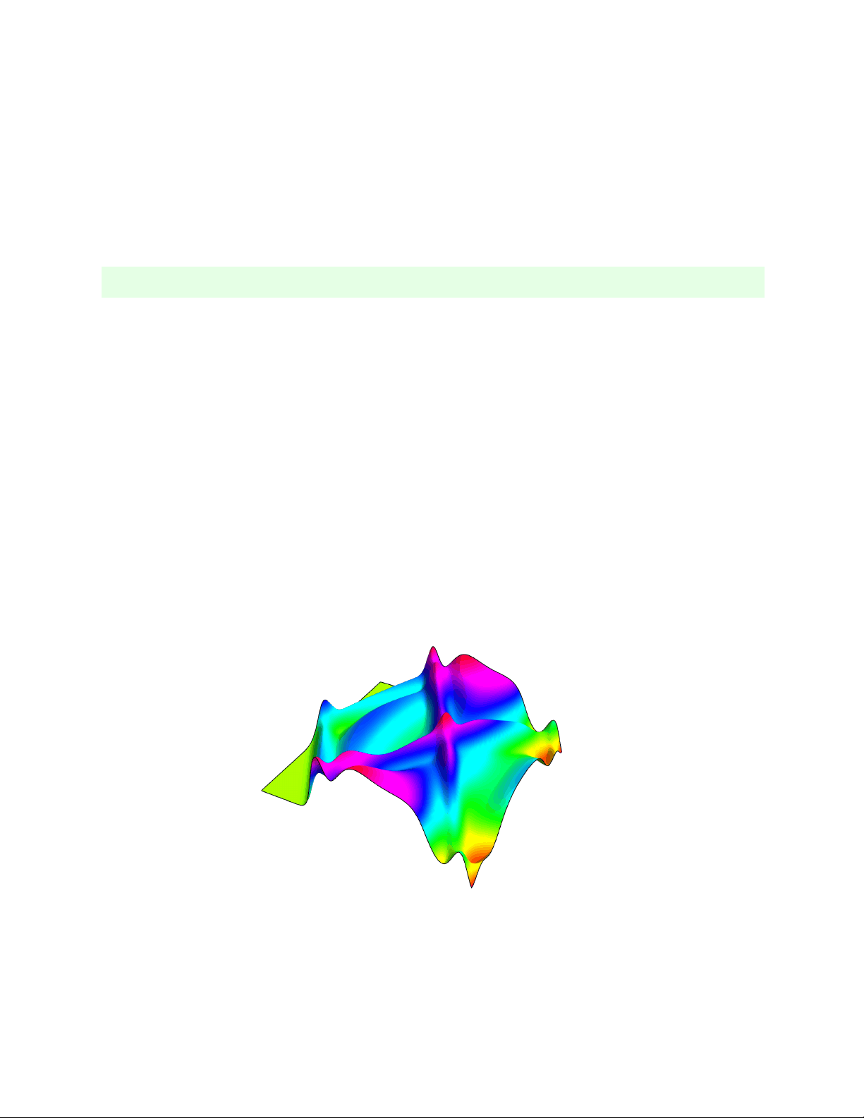
Figure 1. A function f (t, x) satisfying a differential equation ftt − fxx = sin(u). This PDE is called Sin − Gordon equation, a nonlinear wave equation featuring solitons. Space is here one dimensional time goes from left to right. We see a wave going left and right, reflecting at the boundary and building up to a larger peak. A “rogue wave”.
Linear Algebra and Vector Analysis
Lecture
13.2. A partial differential equation is a rule which combines the rates of changes of different variables. Our lives are affected by partial differential equations: the Maxwell equations describe electric and magnetic fields E and B. Their motion leads to the propagation of light. The Einstein field equations relate the metric tensor g with the mass tensor T. The Schr¨odinger equation tells how quantum particles move. Laws like the Navier-Stokes equations govern the motion of fluids and gases and especially the currents in the ocean or the winds in the atmosphere. Partial differential equations appear also in unexpected places like in finance, where for example, the Black-Scholes equation relates the prices of options in dependence of time and stock prices.
13.3. If f (x, y) is a function of two variables, we can differentiate f with respect to both x or y. We just write fx(x, y) for ∂xf (x, y). For example, for f (x, y) = x^3 y + y^2 , we have fx(x, y) = 3x^2 y and fy(x, y) = x^3 + 2y. If we first differentiate with respect to x and then with respect to y, we write fxy(x, y). If we differentiate twice with respect to y, we write fyy(x, y). An equation for an unknown function f for which partial derivatives with respect to at least two different variables appear is called a partial differential equation PDE. If only the derivative with respect to one variable appears, one speaks of an ordinary differential equation ODE. An example of a PDE is f (^) x^2 + f (^) y^2 = fxx + fyy, an example of an ODE is f ′′^ = f 2 − f ′. It is important to realize that it is a function we are looking for, not a number. The ordinary differential equation f ′^ = 3f for example is solved by the functions f (t) = Ce^3 t. If we prescribe an initial value like f (0) = 7, then there is a unique solution f (t) = 7e^3 t. The KdV partial differential equation ft + 6f fx + fxxx = 0 is solved by (you guessed it) 2sech^2 (x − 4 t). This is one of many solutions. In that case they are called solitons, nonlinear waves. Korteweg-de Vries (KdV) is an icon in a mathematical field called integrable systems which leads to insight in ongoing research like about rogue waves in the ocean.
13.4. We say f ∈ C^1 (R^2 ) if both fx and fy are continuous functions of two variables and f ∈ C^2 (R^2 ) if all fxx, fyy, fxy and fyx are continuous functions. The next theorem is called the Clairaut theorem. It deals with the partial differential equation fxy = fyx. The proof demonstrates the proof by contradiction. We will look at this technique a bit more in the proof seminar.
Theorem: Every f ∈ C^2 solves the Clairaut equation fxy = fyx.
13.5. Proof. We use Fubini’s theorem which will appear later in the double integral lecture: integrate
∫ (^) x 0 +h x 0 (
∫ (^) y 0 +h y 0 fxy(x, y)^ dy)dx^ by applying the^ fundamental theorem of calculus twice
∫ (^) x 0 +h x 0 fx(x, y^0 +^ h)^ −^ fx(x, y^0 )^ dx^ =^ f^ (x^0 +^ h, y^0 +^ h)^ −^ f^ (x^0 , y^0 +^ h)^ − f (x 0 +h, y 0 )+f (x 0 , y 0 ). An analogous computation gives
∫ (^) y 0 +h y 0 (
∫ (^) x 0 +h x 0 fyx(x, y)^ dx)dy^ = f (x 0 + h, y 0 + h) − f (x 0 , y 0 + h) − f (x 0 + h, y 0 ) + f (x 0 , y 0 ). Fubini applied to g(x, y) =
fxy(x, y) assures
∫ (^) y 0 +h y 0 (
∫ (^) x 0 +h x 0 fyx(x, y)^ dx)dy^ =^
∫ (^) x 0 +h x 0 (
∫ (^) y 0 +h
∫ ∫ y^0 fyx(x, y)^ dy)dx^ so that A fxy^ −fyx^ dydx^ = 0.^ Assume there is some (x^0 , y^0 ), where^ F^ (x^0 , y^0 ) =^ fxy(x^0 , y^0 )− fyx(x 0 , y 0 ) = c > 0, then also for small h, the function F is bigger than c/2 everywhere on A = [x 0 , x 0 + h] × [y 0 , y 0 + h] so that
A F^ (x, y)^ dxdy^ ≥^ area(A)c/2 =^ h
(^2) c/ 2 > 0 contradicting that the integral is zero.
Linear Algebra and Vector Analysis
Theorem: ftt = fxx is solved by f (t, x) = g(x+t)+ 2 g(x−t)+ h(x+t)− 2 h(x−t).
13.9. Proof. Just verify directly that this indeed is a solution and that f (0, x) = g(x) and ft(0, x) = h(x). Intuitively, if we throw a stone into a narrow water way, then the waves move to both sides. 13.10. The partial differential equation ft = fxx is called the heat equation. Its solution involves the normal distribution N (m, s)(x) = e−(x−m)
(^2) /(2s (^2) ) /
2 πs^2 in probability theory. The number m is the average and s is the standard deviation. 13.11. If the initial heat g(x) = f (0, x) at time t = 0 is continuous and zero outside a bounded interval [a, b], then
Theorem: ft = fxx is solved by f (t, x) =
∫ (^) b a g(m)N^ (m,^
2 t)(x) dm.
Proof. For every fixed m, the function N (m,
2 t)(x) solves the heat equation. � f=PDF[ N o r m a l D i s t r i b u t i o n [m, Sqrt [ 2 t ] ] , x ] ; Simplify [D[ f , t ]==D[ f , { x , 2 } ] ] � �
Every Riemann sum approximation g(x) = (1/n)
∑n k=1 g(mk) of^ g^ defines a function fn(t, x) = (1/n)
∑n k=1 g(mk)N^ (mk,^
2 t)(x) which solves the heat equation. So does f (t, x) = limn→∞ fn(t, x). To check f (0, x) = g(x) which need
−∞ N^ (m, s)(x)^ dx^ = 1 and
−∞ h(x)N^ (m, s)(x)^ dx^ →^ h(m) for any continuous^ h^ and^ s^ →^ 0, proven later. 13.12. For functions of three variables f (x, y, z) one can look at the partial differential equation ∆f (x, y, z) = fxx + fyy + fzz = 0. It is called the Laplace equation and ∆ is called the Laplace operator. The operator appears also in one of the most important partial differential equations, the Schr¨odinger equation
iℏft = Hf = −
ℏ^2
2 m
∆f + V (x)f ,
where ℏ = h/(2π) is a scaled Planck constant and V (x) is the potential depending on the position x and m is the mass. For iℏft = P f with P = −iℏD, then the solution f (x − t) is forward translation. The operator P is the momentum operator in quantum mechanics. The Taylor formula tells that P generates translation.
Homework
Problem 13.1: Verify that for any constant b, the function f (x, t) = e−bt^ sin(x + t) satisfies the driven transport equation ft(x, t) = fx(x, t) − bf (x, t). This PDE is sometimes called the advection equation with damping b.
Problem 13.2: We have seen in class that f (t, x) = e−x (^2) /(4t) /
4 πt solves the heat equation ft = fxx. Verify more generally that e−x (^2) /(4at) /
4 aπt solves the heat equation ft = afxx.
Problem 13.3: The Eiconal equation f (^) x^2 + f (^) y^2 = 1 is used in optics. Let f (x, y) be the distance to the circle x^2 + y^2 = 1. Show that it satisfies the eiconal equation. Remark: the equation can be written rewritten as ||df ||^2 = 1, where df = ∇f = [fx, fy] is the gradient of f which is the Jacobian matrix for the map f : R^2 → R.
Problem 13.4: The differential equation ft = f − xfx − x^2 fxx is a version of the Black-Scholes equation. Here f (x, t) is the price of a call option and x is the stock price and t is time. Find a function f (x, t) solving it which depends both on x and t. Hint: look first for solutions f (x, t) = g(t) or f (x, t) = h(x) and then for functions of the form f (x, t) = g(t) + h(x).
Problem 13.5: The partial differential equation ft + f fx = fxx is called Burgers equation and describes waves at the beach. In higher dimensions, it leads to the Navier-Stokes equation which is used to de- scribe the weather. Verify that the function
f (t, x) =
t
xe−^ x 42 t √ 1 t e
− x 42 t (^) + 1
is a solution of the Burgers equation. You better use technology.
Oliver Knill, knill@math.harvard.edu, Math 22b, Harvard College, Spring 2022