Download Design via Root Locus-Control Systems-Lecture Handout and more Exercises Control Systems in PDF only on Docsity!
N I N E
Design via Root Locus
SOLUTIONS TO CASE STUDIES CHALLENGES
Antenna Control: Lag-Lead Compensation
a. Uncompensated: From the Chapter 8 Case Study Challenge, G(s) =
76.39K
s(s+150)(s+1.32) =
s(s+150)(s+1.32) with the dominant poles at - 0.5 ± j6.9. Hence,^ ζ^ = cos (tan^
0.5 ) = 0.0723, or
%OS = 79.63% and T (^) s =
ζωn
0.5 = 8 seconds. Also, K^ v^ =^
150 x 1.32 = 36.33.
b. Lead-Compensated: Reducing the percent overshoot by a factor of 4 yields, %OS =
19.91%, or ζ = 0.457. Reducing the settling time by a factor of 2 yields, Ts =
2 = 4. Improving
K (^) v by 2 yields K (^) v = 72.66. Using T (^) s =
ζωn
= 4, ζωn = 1, from which ωn = 2.188 rad/s. Thus, the
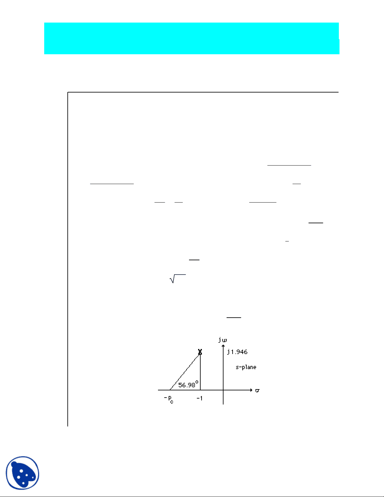
design point equals -ζωn + j ωn 1-ζ^2 = -1 + j1.946. Using the system's original poles and
assuming a lead compensator zero at -1.5, the summation of the system's poles and the lead
compensator zero to the design point is -123.017o^. Thus, the compensator pole must contribute
123.017 o-180 o^ = -56.98 o. Using the geometry below,
p (^) c - 1 = tan 56.^
o, or p (^) c = 2.26.
Adding this pole to the system poles and the compensator zero yields 76.39K = 741.88 at -1+j1.946.
Hence the lead-compensated open-loop transfer function is GLead-comp (s) =
318 Chapter 9: Design Via Root Locus
741.88(s + 1.5)
s(s + 150)(s + 1.32)(s + 2.26)
. Searching the real axis segments of the root locus yields higher-order
poles at greater than -150 and at -1.55. The response should be simulated since there may not be
pole/zero cancellation. The lead-compensated step response is shown below.
Since the settling time and percent overshoot meet the transient requirements, proceed with the lag
compensator. The lead-compensated system has Kv =
741.88 x 1. 150 x 1.32 x 2.26 = 2.487. Since we want K^ v
= 72.66, an improvement of
2.487 = 29.22 is required. Select G(s)^ Lag^ =
s+0. s+0.0001 to improve the
steady-state error by 29.22. A simulation of the lag-lead compensated system,
G (^) Lag-lead-comp(s) =
741.88(s+1.5)(s+0.002922) s(s+150)(s+1.32)(s+2.26)(s+0.0001) is shown below.
320 Chapter 9: Design Via Root Locus
13. No; the feedback compensator's zero is not a zero of the closed-loop system. 14. A. Response of inner loops can be separately designed; B. Faster responses possible; C. Amplification
may not be necessary since signal goes from high amplitude to low.
SOLUTIONS TO PROBLEMS
Uncompensated system: Search along the ζ = 0.5 line and find the operating point is at -1.5356 ±
j2.6598 with K = 73.09. Hence, % OS = e
−ζπ / 1 −ζ 2
x100 = 16.3%; T s =
= 2.6 seconds; Kp
=2.44. A higher-order pole is located at -10.9285.
Compensated: Add a pole at the origin and a zero at -0.1 to form a PI controller. Search along the ζ =
0.5 line and find the operating point is at -1.5072 ± j2.6106 with K = 72.23. Hence, the estimated
performance specifications for the compensated system are: % OS = e
−ζπ / 1 −ζ 2
x100 = 16.3%; T s =
= 2.65 seconds; Kp = ∞. Higher-order poles are located at -0.0728 and -10.9125. The
compensated system should be simulated to ensure effective pole/zero cancellation.
2.
a. Insert a cascade compensator, such as Gc ( s ) =
s + 0.
s
b. Program: K= G1=zpk([],[0,-2,-5],K) %G1=1/s(s+2)(s+5) Gc=zpk([-0.01],[0],1) %Gc=(s+0.01)/s G=G1Gc rlocus(G) T=feedback(G,1) T1=tf(1,[1,0]) %Form 1/s to integrate step input T2=TT t=0:0.1:200; step(T1,T2,t) %Show input ramp and ramp response
Computer response: K =
1
Zero/pole/gain: 1
s (s+2) (s+5)
Solutions to Problems 321
Zero/pole/gain: (s+0.01)
s
Zero/pole/gain: (s+0.01)
s^2 (s+2) (s+5)
Zero/pole/gain:
(s+0.01)
(s+5.064) (s+1.829) (s+0.09593)
(s+0.01126)
Transfer function: 1
s
Zero/pole/gain:
(s+0.01)
s (s+5.064) (s+1.829) (s+0.09593)
(s+0.01126)
a. Searching along the 126.16 o^ line (10% overshoot, ζ = 0.59), find the operating point at
Solutions to Problems 323
Computer response: K =
Zero/pole/gain:
s (s+3) (s+5)
Zero/pole/gain: (s+0.3429)
(s+0.1)
a. Uncompensated: Searching along the 126.16 o^ line (10% overshoot, ζ = 0.59), find the operating
point at -2.03 + j2.77 with K = 45.72. Hence, K (^) p =
2 x 4 x 6 = 0.9525. An improvement of^
= 20.1 is required. Let G (^) c (s) =
0.01. Compensated: Searching along the 126.
o (^) line (10%
overshoot, ζ = 0.59), find the operating point at - 1.99+j2.72 with K = 46.05. Hence, K (^) p =
46.05 x 0. 2 x 4 x 6 x 0.01 = 19.28.
324 Chapter 9: Design Via Root Locus
b.
c. From (b), about 28 seconds
Uncompensated: Searching along the 135 o^ line (ζ = 0.707), find the operating point at
-2.32 + j2.32 with K = 4.6045. Hence, K (^) p =
= 0.153; T (^) s =
= 1.724 seconds; T (^) p =
π
= 1.354 seconds; %OS = e
−ζπ / 1 −ζ 2
x100 = 4.33%;
ωn = 2.32^2 + 2.32^2 = 3.28 rad/s; higher-order pole at -5.366.
Compensated: To reduce the settling time by a factor of 2, the closed-loop poles should be – 4.64 ±
j4.64. The summation of angles to this point is 119 o^. Hence, the contribution of the compensating
zero should be 180o^ -119 o^ =61 o^. Using the geometry shown below,
z c −4.
= tan (61 o). Or, zc = 7.21.
326 Chapter 9: Design Via Root Locus
done=1; while done> a=input('Enter a Test PD Compensator, (s+a). a = ') numc=[1 a]; 'Gc(s)' GGc=tf(conv(numg,numc),deng); GGczpk=zpk(GGc) wn=4/[(estimated_settling_time/2)z]; rlocus(GGc) sgrid(z,wn) title(['PD Compensated Root Locus with ' , num2str(z),... ' Damping Ratio Line', 'PD Zero at ', num2str(a), ', and Required Wn']) done=input('Are you done? (y=0,n=1) '); end [K,p]=rlocfind(GGc); %Allows input by selecting point on graphic 'Closed-loop poles = ' p i=input('Give pole number that is operating point '); 'Summary of estimated specifications' operatingpoint=p(i) gain=K estimated_settling_time=4/abs(real(p(i))) estimated_peak_time=pi/abs(imag(p(i))) estimated_percent_overshoot=pos estimated_damping_ratio=z estimated_natural_frequency=sqrt(real(p(i))^2+imag(p(i))^2) Kp=dcgain(KGGc) 'T(s)' T=feedback(K*GGc,1) 'Press any key to continue and obtain the step response' pause step(T) title(['Step Response for Compensated System with ' , num2str(z),... ' Damping Ratio'])
Computer response: ans =
Uncompensated System
ans =
G(s)
Zero/pole/gain: (s+6)
(s+5) (s+3) (s+2)
Select a point in the graphics window
selected_point =
-2.3104 + 2.2826i
ans =
Closed-loop poles =
p =
-5. -2.3199 + 2.2835i
Solutions to Problems 327
-2.3199 - 2.2835i
Give pole number that is operating point 2
ans =
Summary of estimated specifications
operatingpoint =
-2.3199 + 2.2835i
gain =
estimated_settling_time =
estimated_peak_time =
estimated_percent_overshoot =
estimated_damping_ratio =
estimated_natural_frequency =
Kp =
ans =
T(s)
Transfer function: 4.466 s + 26.
s^3 + 10 s^2 + 35.47 s + 56.
ans =
Press any key to continue and obtain the step response
ans =
Solutions to Problems 329
operatingpoint =
-4.6381 + 4.5755i
gain =
estimated_settling_time =
estimated_peak_time =
estimated_percent_overshoot =
estimated_damping_ratio =
estimated_natural_frequency =
Kp =
ans =
T(s)
Transfer function: 4.75 s^2 + 62.22 s + 202.
s^3 + 14.75 s^2 + 93.22 s + 232.
ans =
Press any key to continue and obtain the step response
330 Chapter 9: Design Via Root Locus
332 Chapter 9: Design Via Root Locus
The uncompensated system performance is summarized in Table 9.8 in the text. To improve settling
time by 4, the dominant poles need to be at -7.236 ± j14.123. Summing the angles from the open-loop
poles to the design point yields -277.326 o. Thus, the zero must contribute 277.326 o^ - 180 o^ = 97.326 o.
Using the geometry below,
s-plane
jω
j14.
-7.236 -zc
97.236o
7.236 - zc = tan(180-97.326). Thus, z^ c^ = 5.42. Adding the zero and evaluating the gain at the design point yields K = 256.819. Summarizing results:
Solutions to Problems 333
a. ζωn =
Ts = 2.5;^ ζ^ =
%OS
π^2 + ln 2 (
%OS
= 0.404. Thus, ωn = 6.188 rad/s and the operating
point is - 2.5 ± j5.67.
b. Summation of angles including the compensating zero is -150.06o. Therefore, the compensator
pole must contribute 150.06 o^ - 180 o^ = -29.94 o.
c. Using the geometry shown below,
p (^) c - 2.5 = tan 29.^
o. Thus, pc = 12.34.
Solutions to Problems 335
tan 48.64 o. Thus, pc = 6.06.
c. Adding the compensator pole and using -2.4 + j4.16 as the test point, K = 29.117.
d. Searching the real axis segments for K = 29.117, we find a higher-order pole at -1.263.
e. Pole at -1.263 is near the zero at -1. Simulate to ensure accuracy of results.
f. K (^) a =
g.
From the plot, Ts = 1.4 seconds; Tp = 0.68 seconds; %OS = 35%.
336 Chapter 9: Design Via Root Locus
a.
-10 -10 -8 -6 -4 -2 0 2
0
2
4
6
8
10
Real Axis
Imag Axis
Uncompensated Root Locus with 0.8 Damping Line
b. and c. Searching along the ζ = 0.8 line (143.13 o), find the operating point at
–2.682 + j2.012 with K = 35.66.
d. Since ζωn =
Ts , the real part of the compensated dominant pole is -4. The imaginary part is
4 tan (180 o-143.13 o) = 3. Using the uncompensated system's poles and zeros along with the
compensator zero at - 4.5, the summation of angles to the design point, -4 + j3 is –158.71o. Thus, the
contribution of the compensator pole must be 158.71 o^ - 180 o^ = -21.29 0. Using the following
geometry,
pc − 4
= tan 21.29 0 , or pc = 11.7.
Adding the compensator pole and using – 4 + j3 as the test point, K = 172.92.
e. Compensated: Searching the real axis segments for K = 172.92, we find higher-order poles at
14.19, and approximately at –5.26 ± j0.553. Since there is no pole/zero cancellation with the zeros at
-6 and –4.5, the system should be simulated to check the settling time.